|
|
|
|
|
|
|
September – November 2013 Quarterly Report |
Dolphin Impact Monitoring |
|
|
|
|
|
|
|
|
|
|
September – November 2013 Quarterly Report |
Dolphin Impact Monitoring |
|
|
|
TABLE
OF CONTENTS
1. Introduction 1
2. Objectives and Methodology 2
2.1. Objectives of the Present Study 2
2.2. Line-transect Vessel Surveys 2
2.2.1 Baseline Survey Data and Data from Impact
Monitoring 3
2.3. Photo-Identification 6
2.4. Data Analyses 6
2.4.1.
Distribution pattern analysis 6
2.4.2.
Encounter rate analysis 6
2.4.3.
Quantitative grid analysis on habitat use 6
2.4.4.
Behavioural analysis 6
2.4.5.
Ranging pattern analysis 7
3. Results and Discussions 7
3.1. Summary of survey effort and dolphin sightings 7
3.2. Distribution 8
3.3. Encounter rate 9
3.4. Group size 10
3.5. Habitat use 10
3.6. Mother-calf pairs 10
3.7. Activities and associations with fishing boats 10
3.8. Photo-identification work and individual range use 11
4. Conclusions 11
5. References 12
Tables
Table
1 The Dolphin Monitoring Transect Co-Ordinates for
HKBCF Monthly
Monitoring 4
Table 2 A Comparison
of Total Sightings Recorded in NEL
and NWL Areas During September–November 2011; 2012; 2013 8
Table 3 A Comparison
of “On Effort” Sightings Recorded in NEL and
NWL Combined During September–November 2011; 2012; 2013 8
Table 4 A Comparison
of “On Effort” Sightings Recorded in NEL and
NWL During September–November 2011; 2012; 2013 9
Table 5 A Comparison of Encounter Rates* in NEL and NWL
Areas
During September–November 2011; 2012; 2013 9
Table 6 A Comparison
of Sightings Group Size Averages Recorded
in NEL and NWL Areas During September–November 2011; 2012; 2013 10
Figures
Figure
1. The
North
Lantau,
Figure
2 Location of the Transect Lines
for Baseline and Impact
Monitoring
during HKBCF (modified to accommodate HKBCF) 5
Figure
3 Distribution of Sightings
Recorded During Impact Monitoring
Surveys
for HKBCF (September 2013) 13
Figure
4 Distribution of Sightings
Recorded During Impact Monitoring
Surveys
for HKBCF (October 2013) 14
Figure
5 Distribution of Sightings
Recorded During Impact Monitoring
Surveys
for HKBCF (November 2013) 15
Figure
6 Distribution of Sightings
Recorded During Impact Monitoring
Surveys
for HKBCF (September – November 2013) 16
Figure 7. The Location of Dolphin Groups Numbering
5 and Above Individuals
(September – November 2013) 17
Figure
8 Sighting density SPSE (number
of on-effort sightings per 100
units
of survey effort) for September – November 2013 18
Figure
9 Dolphin density DPSE (number
of dolphins per 100 units of
survey
effort) for September – November 2013 19
Figure 10. Location of
groups containing mother and calf pairs during
September – November 2013 20
Figure 11. Activity Budget for Dolphin Behaviour
September – November 2013 21
Figure 12. The Location of Different Behavioural
Activities
September – November 2013 22
ANNEXES
Annex I Summary of
Data from the Baseline Monitoring, September – November 2012 and September –
November 2013 and Calculated Encounter Rates
Annex II Impact Monitoring Survey Schedule and Details (September – November 2013)
Annex III Impact Monitoring Survey Effort Summary (September
– November 2013)
Annex IV Impact Monitoring Sighting Database (September
– November 2013)
Annex V Methods Proposal for Density Surface Modelling
and Power Analyses Related to the Hong Kong Zhuhai Macau Bridge (HZMB))
Annex VI Photo ID Images (September – November 2013)
1. Introduction
In March 2012, construction for the Hong Kong-Zhuhai-Macao Bridge
(HZMB) began in

Figure 1.
The Hong Kong Boundary Crossing (HKBCF) Reclamation Sites, North Lantau,
Hong Kong (http://www.hzmb.hk/eng/img/overview/about_overview03_p01l.jpg)
The EM&A Manuals and Environmental Permits (EP) associated with
all three projects have special provision for Chinese white dolphins (CWD) as
they occur regularly in the waters which will be affected by the HZMB
development. This report comprises the
seventh quarterly (September – November 2013)
summary of data associated with the impact monitoring conducted for contract
HY/2010/02, HKBCF-Reclamation Works. The
format of this report follows as closely as possible the outline provided for
the Baseline Monitoring Report. The
baseline monitoring was conducted at the same as this quarter thus three years
of quarterly monitoring can be compared in this report; 2011; 2012 and
2013. Where appropriate, information
from previous reports, data provided by the Hong Kong Highways Department (HyD)
and data from the Agriculture, Fisheries and Conservation Department (AFCD)
Marine Mammal Annual Monitoring reports have also been incorporated[1]
2. OBJECTIVES AND METHODOLOGY
2.1. Objectives of the Present Study
The EM&A Manual for HZMB states that “A dolphin
monitoring programme at North Lantau and West Lantau waters, in particular the
dolphin sighting hotspots (e.g. Brothers Islands) and areas where juveniles
have been sighted (e.g. West Lantau waters), should be set up to verify the
predictions of impacts and to ensure that there are no unforeseen impacts on
the dolphin population during construction phase“. For HKBCF the study area known as
providing ongoing assessment of the spatial and temporal distribution
patterns and habitat use of CWD during the construction phase of the HKBCF
project.
identifying individual CWD by their natural marks, coloration and
scars for comparison with the baseline data and to assess individual
distribution patterns and habitat use.
comparing impact survey data to that gathered during the baseline
data period so that any changes deemed to be of a significant nature can be
assessed and mitigated appropriately.
The baseline monitoring report includes distribution analysis,
encounter rate analysis, behavioural analysis, quantitative grid analysis and
ranging pattern analysis. Protocols for
data interpretation and analyses methods were provided in the baseline monitoring
report.
2.2. Line-transect Vessel Surveys
The co-ordinates for
the transect lines and layout map were provided by AFCD, however, these have
been modified as the construction works at HKBCF has shortened one of the
transect lines (Table 1; Figure 2). The
study area now incorporates 23 transects (totalling ~111km) which are surveyed
twice per month by boat. Line transect
surveys should be conducted systematically and lines travelled in sequence
(Buckland et al 2001). When the start of a transect line is reached,
“on effort” survey begins. When the
vessel is travelling between transect lines and to and from the study area, it
is deemed to be “off effort”. The
transect line is surveyed at a speed of 7-8 knots (13-15 km/hr). During some periods, tide and current flow in
the study site exceeds 7 knots and thus the vessel travels at the same speed as
the current during these periods. A
minimum of four marine mammal observers (MMOs) are present on each survey,
rotating through four positions; observers (2), data recorder (1) and rest
(1). Rotations occur every 30 minutes or
at the end of dolphin sightings. The
data recorder enters vessel effort, observer effort, weather and sightings
information directly onto the programme Logger[2] and is not part of the observer team. This is not standard line transect survey
procedure, however, the baseline study was conducted this way thus it has been
requested that only two observers be used for impact surveys.
When the boat is travelling along
the transect line (“on effort”), observers search the area in front of the boat
between 90° and 270° abeam (bow being 0°).
When a group of dolphins is sighted, position, bearing and distance data
are recorded immediately onto Logger and, after a short observation, an
estimate is made of group size[3]. This is an “on effort” sighting. These input parameters are linked to the
time-GPS-ships data which are automatically stored in Logger throughout the
survey period. In this manner,
information on heading, position, speed, weather, effort and sightings are
stored in an interlinked database which can be subsequently used in a variety
of analytical software packages.
Once the
vessel leaves the transect line, it is deemed to be “off-effort”. The dolphins are approached with the purpose
of taking high resolution images. Then
the vessel returns to the transect line at the point of departure and is again
“on effort”. If another group of
dolphins is seen while travelling back to the transect line, or when with the
first group of dolphins, the sightings are considered as “opportunistic” and
noted accordingly.
2.2.1 Baseline
Survey Data and Data from Impact Monitoring
Data from the baseline was provided by the Highways
Department (January 2013) and data has been reported monthly throughout the
impact monitoring period. For ease of reference, these data have been
summarised from that previously reported and encounter rate calculations are
provided (Annex I).
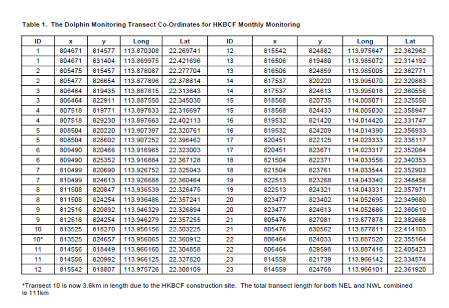
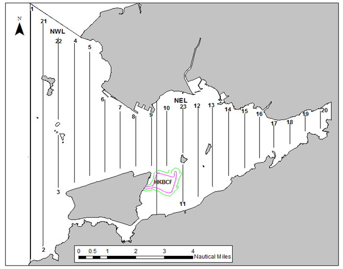
Figure 2 Location of
the Transect Lines for Baseline and Impact Monitoring during HKBCF (modified to
accommodate HKBCF)
2.3. Photo-identification
When a dolphin(s) is sighted, the vessel
leaves the transect line and slowly approaches the group or individual. Attempts are made to photograph every
individual sighted although close approaches to mother and calf pairs are not
attempted. A digital SLR camera (Nikon
D90) using long lenses (Nikor 80-200mm and fixed length 300mm) are used to
obtain high resolution images. Effort is
made to ensure consistency of image quality, e.g., no shadow and at an angle
perpendicular to the dorsal fin.
Polarising filters are used to minimise glare. In this manner, the best image clarity is
achieved and image sorting and matching is more consistent. Images are sorted
according to clarity and presence/absence of identifying features
(nicks/cuts/deformities/injury/pigmentation).
Only images deemed to be of suitable quality and as containing
sufficient markings for unambiguous identification are included in the
photo-identification catalogue.
2.4. Data Analyses
2.4.1. Distribution pattern analysis
Dolphin sightings data are mapped in the Geographic Information
System (GIS) ArcView© 10.1.
2.4.2. Encounter rate analysis
For this report, the baseline encounter rates were re-calculated using the revised data
provided (as presented in Annex I) rather than quoting directly from the
baseline report. Calculation followed
the EM&A Manuel methodology (“on-effort” sightings made during favourable
weather and visibility conditions).
2.4.3. Quantitative grid analysis of habitat use
Quantitative grid
analysis is performed by mapping both sighting and dolphin densities plotted
onto 1kmx1km grid squares. Only “on
effort” sightings made while on a transect line and under favourable conditions
should be included in grid analyses.
These densities are standardised by effort by calculating survey
coverage in each line transect survey to determine the number of times the grid
has been surveyed. Densities are
calculated using the following formulae;
SPSE and DPSE:
SPSE = (S/E x 100)/SA%
DPSE = (D/E x 100)/SA%
Where;
S= total number “on
effort” sightings
D = total number
dolphins from “on effort” sightings
E = total number units
survey effort
SA% = percentage of sea
area
2.4.4. Behavioural analysis
When dolphins are sighted during vessel surveys, their behaviour is
observed. Different activities are categorised (i.e. feeding, traveling,
surface active, associated with boats, unknown) and recorded in the sighting
data form of Logger. The sightings form
is integrated with survey effort and positional data and can be subsequently
mapped to examine distribution and behavioural trends. All sightings data (“on-effort” and
“opportunistic”) are used in this analysis.
2.4.5. Ranging pattern analysis
Home ranges for individual dolphins can be calculated using a variety
of software (Worton 1989). In the
baseline monitoring report, the program Animal Movement Analyst Extension,
created by the Alaska Biological Science Centre, USGS was used in conjunction
with ArcView© 3.1 and Spatial Analyst 2.0.
Using the fixed kernel method, kernel density estimates and kernel
density plots are created using all sightings.
In the baseline monitoring, data from other studies and from outside the
baseline monitoring period were used to map individual ranges. It is important to maximize the number of
sightings used as kernel analyses cannot be conducted unless more than 20
independent sightings are made for an individual although it is recommended
that a minimum of 70 resightings are used before kernel analyses has any
accuracy (Wauters et al 2007; Kauhala
and Auttila 2010). AFCD Annual Reports
use a minimum of 15 resightings for kernel analyses (AFCD 2012). To date, too few data on individual dolphins
exist from impact monitoring alone, i.e., 15 or more independent resightings
per individual, to map utilisation densities using the fixed kernel
method. The most resightings for an
individual dolphin in the baseline and impact monitoring period combined is
thirteen (HZMB 054) split across baseline (seven sightings) and impact
monitoring (6 sightings). A comparison
of baseline and impact sightings using kernel analyses will require longer term
data collection.
3. RESULTS AND DISCUSSIONS
3.1. Summary of survey effort and dolphin sightings
From September – November, 12 vessel surveys were conducted in NEL and NWL survey areas (Annex
II). A total of 668.2 km of “on-effort”
transect lines were conducted, of which 665.9km were under favourable
conditions. Therefore, 99.7% of vessel
surveys were conducted under favorable conditions (Annex III). Only those periods of “on-effort” survey
conducted under favourable conditions were included in quantitative
analyses. During September – November 2013,
42 groups of dolphins, numbering 133 (min 131: max 143[4]) individuals, were sighted from the vessel surveys. Of these, 28 groups were “on-effort” and the
remaining 14 “opportunistic” (Annex IV).
Of the 42 sightings,
41 groups were located in NWL and 1 in NEL.
The baseline report, conducted during September-November 2011, notes a
total of 44 groups, 34 of which occurred in NWL and 10 in NEL. For period September – November 2012,
a total of 71 groups were sighted, 53 of which were located in NWL and 18 in
NEL. There are differences between the number of sightings made during baseline
compared to the same period in 2012 and 2013.
For NEL, the number of groups almost doubled between baseline (2011) and
September – November 2012 and then decreased markedly in September – November
2013. For NWL, both September – November
2012 and 2013 recorded larger numbers of groups when compared to baseline
monitoring (Table 2). Maps depicting
location of sightings which have not been corrected for effort or survey track
length are included as Figs. 3;4;5;6.
Table
2. A Comparison of Total Sightings
Recorded in NEL and NWL Areas During Sep – Nov 2011; 2012 and 2013
|
Monitoring Period |
Total Dolphin Sighting in NWL |
Total Dolphin Sighting in NEL |
|
Number of Groups |
Number of Groups |
|
|
Sep – Nov 2011* (Baseline Monitoring) |
34 |
10 |
|
Sep – Nov 2012* (HKBCF Third Quarter) |
53 |
18 |
|
Sep – Nov 2013* (HKBCF Seventh Quarter) |
41 |
1 |
* All
Surveys conducted once per month
As per the EM&A
manual, only “on effort” sightings can be used for some analyses therefore the
combined number of “on effort” sightings for all three periods was compared
There is an increase in the total number of “on effort” sightings between
baseline monitoring (2011) and impact monitoring (2012) but a decrease below
both previous totals in September – November 2013 (Table 3). No correction for effort
is made with these numbers, this is calculated in section 3.3.
Table 3.
A Comparison of “On Effort” Sightings Recorded in NEL and NWL Combined
During Sep – Nov 2011; 2012 and 2013.
|
Monitoring Period |
Groups of Dolphin sighted in NEL and NWL |
|
Sep
- Nov 2011 (Baseline
Monitoring) |
44 |
|
Sep – Nov
2012 (HKBCF
Third Quarter) |
52 |
|
Sep – Nov
2013 (HKBCF
Seventh Quarter) |
28 |
3.2. Distribution
During the both the baseline survey and the same period the following
year, approximately three quarters of all “on effort” sightings were made in
NWL. For the period September – November
2013, however, no “on effort” sightings were made in NEL. The similarity between the 2011 and 2012
periods is noted, however, there is no correction for effort (Table 4). Throughout September – November 2013, the
area of most use was the northern section of NWL, within and adjacent to the
Shau Chau and Lung Kwu Chau Marine Park (SCLKCMP). A few groups were recorded at the Tai O area
and only two groups at the E edge of the airport platform. Only one group was recorded in NEL at the
east of the Brothers Islands (Fig. 6).
These areas are highlighted consistently throughout AFCD annual
monitoring reports as well as during pre construction monitoring. SCLKCMP is frequented all year round by
dolphins and is perceived to be critical habitat whereas the use of NEL is
regarded as more seasonal, however, the decrease in the number of groups
occurring in NEL compared to the same season in previous years is
noteworthy.
Table 4.
A Comparison of “On Effort” Sightings Recorded in NEL and NWL During Sep
– Nov 2011; 2012 and 2013.
|
Monitoring Period |
No. of Dolphin Groups sighted in NWL |
No. of Dolphin Groups sighted in NEL |
|
Sep - Nov 2011
(Baseline Monitoring) |
34 |
10 |
|
Sep – Nov
2012 (HKBCF
Third Quarter) |
39 |
13 |
|
Sep – Nov
2013 (HKBCF
Seventh Quarter) |
28 |
0 |
3.3. Encounter rate
As the survey periods have different transect lengths, variation in
sightings occurrence was quantified by correcting for the different amount of
effort (number and distance of transect lines surveyed, i.e., km spent
“on-effort”), to obtain an encounter rate.
The baseline study (Sep-Nov 2011) reports that a total of 545.6km[5] of survey effort was conducted under favourable conditions in the
NEL and NWL survey areas. In NEL and NWL
combined, 659.8km and 665.9km of track-line were conducted under favourable
conditions during the periods September – November 2012 and 2013,
respectively. In NEL, there is a slight
increase in encounter rate between baseline and the same period the following
year, however, for the period September – November 2013, there is a marked decrease
in encounter rate. i.e., 6.3 to 0. For
NWL, there is a continuous decline in encounter rate from the baseline period
through the same period the next and subsequent years, i.e., 9.5 to 8.7 to 6.3
(Table 5).
Table
5. A Comparison of Encounter Rates*
in NEL and NWL Areas During September-November 2011; 2012 and 2013.
|
Monitoring Period |
Encounter Rate NEL |
Encounter Rate NWL (*) |
|
Sept-Nov
2011 (Baseline
Monitoring) |
5.4 |
9.5 |
|
Sep – Nov
2012 (HKBCF
Third Quarter) |
5.9 |
8.9 |
|
Sep – Nov
2013 (HKBCF
Seventh Quarter) |
0 |
6.3 |
The AFCD Annual
Reports describe variation in spatial distribution between areas and between
seasons in NEL and NWL. For the last
sixteen years, it is reported that overall annual
encounter rate for NEL varies between 1.6 and 6.2 and the annual encounter rate for NWL varies
between 5.8 and 17.0. The encounter rate
for NWL for all three periods (September – November 2011; 2012; 2013) is within
the annual limits recorded for this area previously. For NEL, the encounter rates in September –
November 2011 and 2012 are within the recorded annual norms for the area,
however, the encounter rate of zero for the same period 2013 is not. Historically, there have been both up and
down movements within these limits, however, the general trend in yearly
encounter rate for dolphins in all areas of Hong Kong is that of significant
decline over the last decade and prior to new development projects in the
Lantau area (AFCD 2013). The known
decline in the population, on top of the highly variable encounter rate noted
historically, makes it problematic to discern any additional influence
individual projects, such as HKBCF and others, may have on the dolphin
population encounter rate. As the impact
of the work at HKBCF extends in addition to new dredging and other projects
being initiated in NEL, it is likely that these activities have effected NEL
encounter rates.
3.4. Group size
During September – November 2013, group size of all sightings varied
from 1 to 12 individuals with an average of 3.2 in NWL and 1 in NEL. For baseline monitoring, the NWL average
group size was 4.5 and the NEL average group size was 3.5. For the period September 2012, the NWL
average group size was 3.1 and in NEL it was 3.6 (Table 6). NEL shows a decreased number in groups size (although
it is noted only one group was sighted in September – November 2013). In NWL, groups sizes between September –
November 2012 and 2013 are approximately the same although both are lower than
the baseline monitoring. A map depicting
group size distribution shows that the two largest groups occurred at SCLKCMP
and both of these groups contained calves (Fig. 7).
Table 6. A
Comparison of Sightings Group Size Averages Recorded in NEL and NWL Areas
During Sep – Nov 2011; 2012 and 2013
|
Monitoring Period |
Average Group Size (NWL) |
Average Group Size (NEL) |
|
|
Sep - Nov 2011 (Baseline Monitoring) |
4.5 |
3.5 |
|
|
Sep – Nov
2012 (HKBCF
First Quarter) |
3.1 |
3.6 |
|
|
Sep – Nov
2013 (HKBCF
Seventh Quarter) |
3.2 |
1.0 |
|
As encounter rate and group size are both
subject to variation, the use of other more powerful analyses may be more
appropriate to discern differences over the shorter term, such as multi-variate
analyses (Taylor et al 2007). This is important so that project impact can
be monitored over relevant time scales.
Alternative analyses have been proposed and developed using the first
year of impact monitoring data and the methodology is attached (Annex V). Considerable reformatting of baseline data
and incorporation of environmental and habitat data from multiple sources is
near completion and the models will be run over the next quarterly period [6]
3.5. Habitat use
Quantitative grid analyses indicates that the most often frequented
areas in NWL were the SCLKCMP, the western limit of NWL and one area to the
north of the Hong Kong International Airport (HKIA) platform. In NEL, no “on effort” sightings occurred
therefore no qualitative grid analyses can be conducted (Figs. 8; 9). The grid analyses from this quarter shows a
similar distribution in NWL to that published in the AFCD long term monitoring
reports and the baseline monitoring report.
These areas of high use have been consistent in the long term and
continue to be so. The decrease in
dolphin sightings between September – November 2013 and the two previous autumn
seasons is noted. It is also noted that
the areas of DPSE and SPSE which were apparent in summer 2013 are also absent.
3.6. Mother-calf pairs
Seven of the groups sighted contained mother and calf pairs[7]. All groups were sighted in
NWL (Fig. 10). Calves comprised 6.7% of
all dolphins sighted, much higher than that reported in the last quarterly
report (2.5%). Although calf mortality
was highlighted in previous seasons, several new born dolphins have been
sighted consistently in NWL this quarter.
3.7. Activities
Of the 42 groups sighted (using all sightings), 21 (50%) were engaged
in feeding activities; three (7%) were travelling; 11 (26%) were
feeding/travelling/surface active; two (5%) were milling (other) and it was not
possible to define the behavior of five (12%) groups. Feeding was the predominant activity during
daylight hours in September – November 2013 with travelling/feeding/surface
active (multiple) behaviours being the next most dominant behavioural category
(Fig. 11). In NWL, feeding occurred most
often at east SCLKCMP and the western limits of NWL. (Fig. 12).
3.8. Photo-identification work
The photo-identification catalogue was
regularly updated and re-sightings of dolphins previously identified were
recorded. The project specific
photo-identification catalogue for the impact monitoring period is presented in
Annex VI. Not all dolphins sighted have
sufficient scarring, injury or pigmentation uniqueness to be unambiguously
identified. During the baseline survey, 96 individuals were noted in the NEL,
NWL and WL areas. Of these, 57 were
noted in the NEL and NWL area. No new
dolphins which have been identified in the last quarter are from the baseline
study, however, several well known individuals have been recorded throughout
September – November 2013. There are
five dolphins which have been sighted more than seven times, all of which are
known from the AFCD catalogue (HZMB 002 [WL111]; HZMB 011 [EL01]; HZMB 041
[NL24]; HZMB 044 [NL98]; HZMB054 [CH34]).
Two of these well known individuals were not seen during the baseline
study (HZMB 002 AND HZMB 044). When both
baseline and impact monitoring data is pulled, HZMB 54 has been seen the most
in 14 different sighting groups. HZMB 041 has been sighted 11 times; HZMB 002 has been
sighted ten times, HZMB 044 has been sighted nine times and HZMB 011 has been
sighted eight times. Even when pooled with baseline data, the highest number of
re-sightings is 14 (HZMB 054) and this does not consider independence of
sightings, a critical assumption in kernel analyses. (Annex VI; Table1).
4. CONCLUSION
The data from September – November 2013
shows some consistencies with the results reported in the same period 2011
(baseline) and 2012. Habitat use,
encounter rates, group size and behavioural trends all fall within those
reported in AFCD Long Term Monitoring reports apart from the use of NEL which
has dropped when compared to this season in previous years. It is noted from the previous quarterly
report which summaries the summer seasons for the last three years, there was
an increase in seasonal usage of NEL.
Density distribution maps depicted key areas of frequent use within NWL,
in particular, SCLKMP and Tai O.
Behavioural patterns were broadly similar, with feeding behavior
predominating all months. .
The
decrease in encounter rate in NEL is noted although no link can be found
between this and specific activities at HKBCF.
Although it is likely that the increase in HKBCF activities is having an
effect on dolphin encounter rates in NEL (although not in the three months that
preceded this quarter), it is also noted that a dredging project was started in
November 2013 and new project works also were initiated in NEL during the
autumn of 2013. Increased activities in
addition to the inherent variation apparent in dolphin distribution and habitat
use make it challenging to discern specific sources of impact. A significant decline in dolphin throughout
the last ten years prior to construction commencement has also been published
by AFCD (2013). It is hoped that the
fine scale density surface analysis presently being conducted will allow
further light to be shed on the specific areas and environmental variables,
including marine construction works, which impacts dolphin distribution
throughout NEL and NWL.
References
Agriculture, Fisheries and Conservation Department (AFCD) 2012. Annual Marne Mammal Monitoring Programme
April 2011-March 2012. ) The Agriculture, Fisheries and Conservation
Department, Government of the Hong Kong SAR.
Buckland, S., Burnham, K., Laake, J., Borchers, D. and Thomas, L.
2001. Introduction to Distance Sampling.
Oxford University Press.
Connor, R. Mann, J., Tyack, P. and Whitehead, H. 1998. Social
Evolution in Toothed Whales. Trends in
Ecology and Evolution 13, 228-232
Gillespie,
D., Leaper, R., Gordon, J. and Macleod, K. 2010. An
integrated data collection system for line transect surveys. J. Cetacean Res. Manage. 11(3): 217–227.
Kauhala, K. & Auttila, M. 2010:
Estimating habitat selection of badgers - a test between different methods. - Folia
Zoologica 59: 16-25.
Taylor, B., Martinez, M, Gerodette, T., Barlow, J and Hrovat, Y. 2007.
Lessons from Monitoring Trends in Abundance of Marine Mammals. Marine
Mammal Science 23(1):157-175.
Wauters, L., Preatoni, D., Molinari, A. and
Tosi, G. 2007. Radio-tracking squirrels: Performance of home range density and
linkage estimators with small range and sample size. Ecological Modelling
202(10):333-44
Worton, B. 1989. Kernel
Methods for Estimating Utilization Distribution in Home Range Studies. Ecology 70(I):164-8
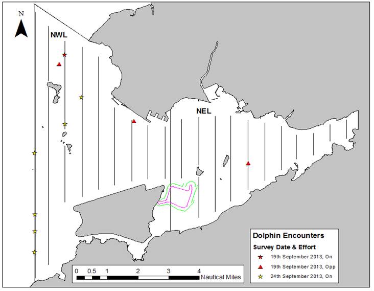
Figure 3 Distribution of Sightings Recorded During Impact Monitoring
Surveys for HKBCF (September 2013)
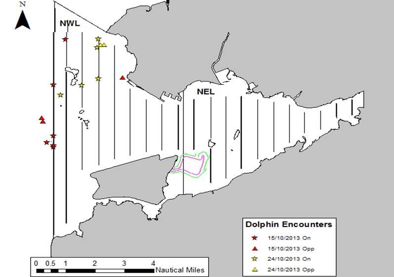
Figure
4 Distribution of Sightings Recorded During Impact Monitoring Surveys for HKBCF
(October 2013)
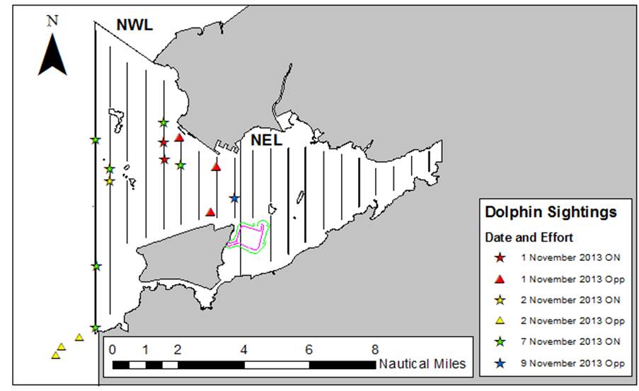
Figure 5 Distribution of Sightings Recorded During Impact Monitoring
Surveys for HKBCF (November 2013)
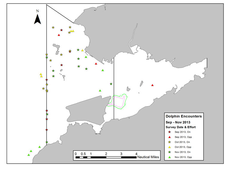
Figure 6. Distribution of Sightings Recorded During Impact Monitoring
Surveys for HKBCF (September – November 2013)
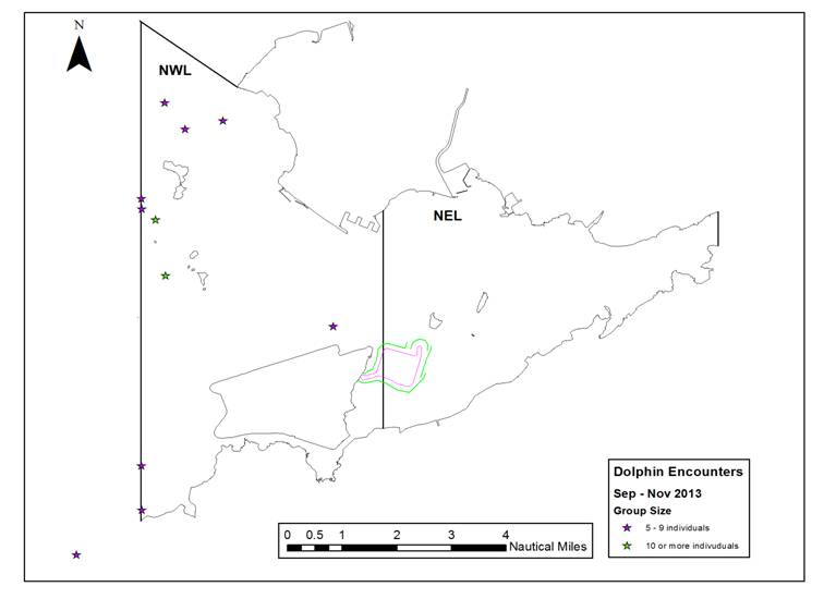
Figure 7. The Location of Dolphin Groups Numbering 5 and Above
Individuals (September – November 2013)
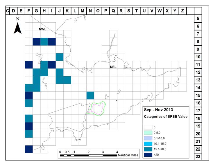
Figure 8. Sighting density SPSE (number of on-effort sightings per
100 units of survey effort) for September – November 2013.
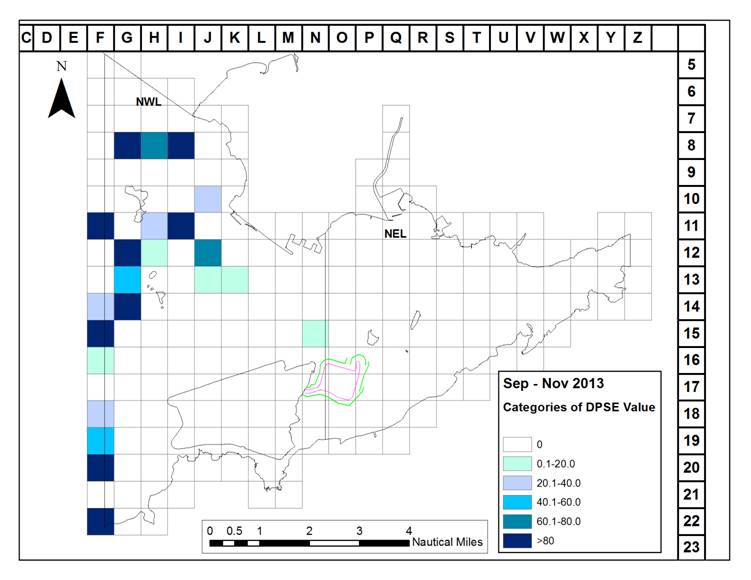
Figure 9. Dolphin density DPSE (number of dolphins per 100 units of
survey effort) for September – November 2013.
![]()
![]()
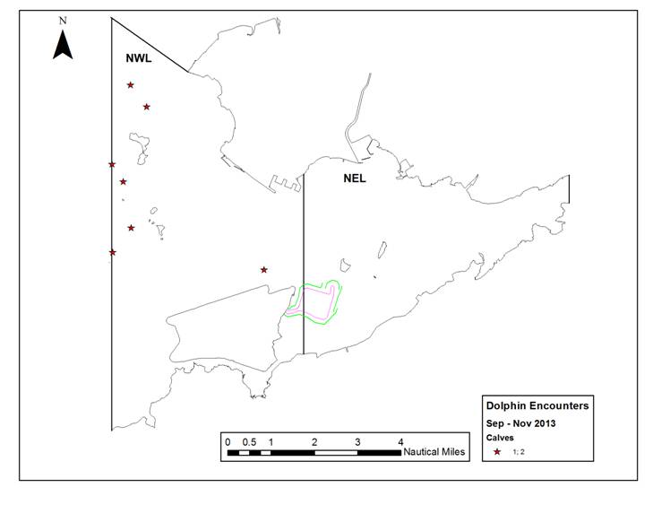
Figure 10. Location of groups
containing mother and calf pairs during September – November 2013.

Figure 11. Activity Budget for Dolphin Behaviour September
– November 2013.
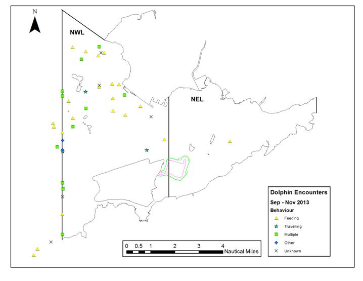
Figure 12. The Location of Different Behavioural Activities June to
August 2103
Annex
I Summary of Data from the Baseline Monitoring and September – November 2012
and September – November 2013 (this study) and Calculated Encounter Rates
|
Date |
Area |
Groups |
Trackline
(KM) |
Encounter
rate |
|
Sept
– Nov 2011 (Baseline
Monitoring) |
NEL |
10 |
175.7 |
5.4 |
|
Sept
– Nov 2011 (Baseline
Monitoring) |
NWL |
34 |
359.0 |
9.5 |
|
Sept-Nov
2012 (Third
Quarter) |
NEL |
13 |
221 |
5.9 |
|
Sept-Nov
2012 (Third
Quarter) |
NWL |
39 |
438.8 |
8.9 |
|
Sept-Nov
2013 (Seventh
Quarter) |
NEL |
0 |
220.7 |
0 |
|
Sept-Nov
2013 (Seventh
Quarter) |
NWL |
28 |
445.2 |
6.3 |
Annex II. Impact Monitoring Survey Schedule and
Details (September – November 2013)
|
Date |
Location |
No. Sightings “on effort”
|
No. Sightings
“opportunistic” |
Total km “on effort” |
|
17/09/2013 |
NE Lantau |
0 |
0 |
33.5 |
|
19/09/2013 |
NW & NE Lantau |
1 |
3 |
77.5 |
|
24/09/2013 |
NW Lantau |
6 |
0 |
63.4 |
|
25/09/2013 |
NW & NE Lantau |
0 |
0 |
47.6 |
|
15/10/2013 |
NW Lantau |
6 |
3 |
59.7 |
|
17/10/2013 |
NW & NE Lantau |
0 |
0 |
52.1 |
|
24/10/2013 |
NW Lantau |
5 |
2 |
58.7 |
|
28/10/2013 |
NW & NE Lantau |
0 |
0 |
51.8 |
|
01/11/2013 |
NE and NW Lantau |
2 |
3 |
59.5 |
|
02/11/2013 |
NWL |
1 |
3 |
52.2 |
|
07/11/2013 |
NWL |
6 |
0 |
64.7 |
|
09/11/2013 |
NE and NW Lantau |
1 |
0 |
47.5 |
|
Total |
28 |
14 |
668.2 |
All
effort in all sea states is listed
Annex III. Impact Monitoring Survey Effort Summary
(September – November 2013)
|
Date |
Area |
Beaufort |
Effort
(km) |
Season |
Vessel |
Type |
|
|
17/9/2013 |
NEL |
1 |
9.2 |
AUTUMN |
HKDW |
IMPACT |
|
|
17/9/2013 |
NEL |
2 |
15.6 |
AUTUMN |
HKDW |
IMPACT |
|
|
17/9/2013 |
NEL |
3 |
7.7 |
AUTUMN |
HKDW |
IMPACT |
|
|
17/9/2013 |
NEL |
4 |
1 |
AUTUMN |
HKDW |
IMPACT |
|
|
19/9/2013 |
NEL |
2 |
3.5 |
AUTUMN |
HKDW |
IMPACT |
|
|
19/9/2013 |
NWL |
1 |
10.6 |
AUTUMN |
HKDW |
IMPACT |
|
|
19/9/2013 |
NWL |
2 |
44.7 |
AUTUMN |
HKDW |
IMPACT |
|
|
19/9/2013 |
NWL |
3 |
18.7 |
AUTUMN |
HKDW |
IMPACT |
|
|
24/9/2013 |
NWL |
1 |
23.6 |
AUTUMN |
HKDW |
IMPACT |
|
|
24/9/2013 |
NWL |
2 |
19.4 |
AUTUMN |
HKDW |
IMPACT |
|
|
24/9/2013 |
NWL |
3 |
20.4 |
AUTUMN |
HKDW |
IMPACT |
|
|
25/9/2013 |
NWL |
1 |
7.6 |
AUTUMN |
HKDW |
IMPACT |
|
|
25/9/2013 |
NWL |
2 |
2.7 |
AUTUMN |
HKDW |
IMPACT |
|
|
25/9/2013 |
NEL |
1 |
20.3 |
AUTUMN |
HKDW |
IMPACT |
|
|
25/9/2013 |
NEL |
2 |
17 |
AUTUMN |
HKDW |
IMPACT |
|
|
15/10/2013 |
NWL |
1 |
35.8 |
AUTUMN |
HKDW |
IMPACT |
|
|
15/10/2013 |
NWL |
2 |
23.9 |
AUTUMN |
HKDW |
IMPACT |
|
|
17/10/2013 |
NWL |
1 |
1.1 |
AUTUMN |
HKDW |
IMPACT |
|
|
17/10/2013 |
NWL |
2 |
7.4 |
AUTUMN |
HKDW |
IMPACT |
|
|
17/10/2013 |
NWL |
3 |
6 |
AUTUMN |
HKDW |
IMPACT |
|
|
17/10/2013 |
NEL |
1 |
9.2 |
AUTUMN |
HKDW |
IMPACT |
|
|
17/10/2013 |
NEL |
2 |
20.5 |
AUTUMN |
HKDW |
IMPACT |
|
|
17/10/2013 |
NEL |
3 |
7.9 |
AUTUMN |
HKDW |
IMPACT |
|
|
24/10/2013 |
NWL |
1 |
12.2 |
AUTUMN |
HKDW |
IMPACT |
|
|
24/10/2013 |
NWL |
2 |
32.7 |
AUTUMN |
HKDW |
IMPACT |
|
|
24/10/2013 |
NWL |
3 |
13.7 |
AUTUMN |
HKDW |
IMPACT |
|
|
24/10/2013 |
NWL |
4 |
0.1 |
AUTUMN |
HKDW |
IMPACT |
|
|
28/10/2013 |
NWL |
1 |
4.9 |
AUTUMN |
HKDW |
IMPACT |
|
|
28/10/2013 |
NWL |
2 |
10.2 |
AUTUMN |
HKDW |
IMPACT |
|
|
28/10/2013 |
NEL |
1 |
14.6 |
AUTUMN |
HKDW |
IMPACT |
|
|
28/10/2013 |
NEL |
2 |
10.7 |
AUTUMN |
HKDW |
IMPACT |
|
|
28/10/2013 |
NEL |
3 |
11.4 |
AUTUMN |
HKDW |
IMPACT |
|
|
11/1/2013 |
NEL |
1 |
35.4 |
AUTUMN |
HKDW |
IMPACT |
|
|
11/1/2013 |
NWL |
1 |
14.6 |
AUTUMN |
HKDW |
IMPACT |
|
|
11/1/2013 |
NWL |
2 |
9.5 |
AUTUMN |
HKDW |
IMPACT |
|
Annex III. Impact Monitoring Survey Effort Summary
(September – November 2013) (con) |
||||||
|
Date |
Area |
Beaufort |
Effort (km) |
Season |
Vessel |
Type |
|
11/2/2013 |
NWL |
2 |
26.7 |
AUTUMN |
HKDW |
IMPACT |
|
11/2/2013 |
NWL |
3 |
24.3 |
AUTUMN |
HKDW |
IMPACT |
|
11/2/2013 |
NWL |
4 |
1.2 |
AUTUMN |
HKDW |
IMPACT |
|
11/7/2013 |
NWL |
1 |
43.4 |
AUTUMN |
HKDW |
IMPACT |
|
11/7/2013 |
NWL |
2 |
21.3 |
AUTUMN |
HKDW |
IMPACT |
|
11/9/2013 |
NEL |
1 |
10 |
AUTUMN |
HKDW |
IMPACT |
|
11/9/2013 |
NEL |
2 |
21.2 |
AUTUMN |
HKDW |
IMPACT |
|
11/9/2013 |
NEL |
3 |
6.5 |
AUTUMN |
HKDW |
IMPACT |
|
11/9/2013 |
NWL |
1 |
3.7 |
AUTUMN |
HKDW |
IMPACT |
|
11/9/2013 |
NWL |
2 |
6.1 |
AUTUMN |
HKDW |
IMPACT |
Annex IV. Impact Monitoring Sighting Database (September – November
2013)
|
Project |
Contract |
Date |
Sighting No. |
Time |
Group Size |
Area |
Beaufort |
PSD |
Effort |
Type |
Latitude |
Longitude |
Season |
Boat Assoc |
|
HKBCF |
HY/2010/02 |
9/19/2013 |
791 |
9:42 |
1 |
NEL |
1 |
NA |
Opp |
Impact |
22.33573 |
113.9952 |
Autumn |
No |
|
HKBCF |
HY/2010/02 |
9/19/2013 |
792 |
11:31 |
1 |
NWL |
2 |
NA |
Opp |
Impact |
22.35992 |
113.9283 |
Autumn |
No |
|
HKBCF |
HY/2010/02 |
9/19/2013 |
794 |
14:13 |
4 |
NWL |
2 |
94 |
On |
Impact |
22.39786 |
113.8874 |
Autumn |
No |
|
HKBCF |
HY/2010/02 |
9/19/2013 |
795 |
14:31 |
6 |
NWL |
2 |
NA |
Opp |
Impact |
22.39240 |
113.8843 |
Autumn |
No |
|
HKBCF |
HY/2010/02 |
9/24/2013 |
798 |
9:19 |
5 |
NWL |
1 |
243 |
On |
Impact |
22.28493 |
113.8701 |
Autumn |
No |
|
HKBCF |
HY/2010/02 |
9/24/2013 |
799 |
10:02 |
1 |
NWL |
1 |
279 |
On |
Impact |
22.29694 |
113.8703 |
Autumn |
No |
|
HKBCF |
HY/2010/02 |
9/24/2013 |
800 |
10:15 |
2 |
NWL |
1 |
30 |
On |
Impact |
22.30655 |
113.8702 |
Autumn |
No |
|
HKBCF |
HY/2010/02 |
9/24/2013 |
802 |
10:42 |
2 |
NWL |
2 |
78 |
On |
Impact |
22.34161 |
113.8700 |
Autumn |
No |
|
HKBCF |
HY/2010/02 |
9/24/2013 |
803 |
13:33 |
1 |
NWL |
1 |
221 |
On |
Impact |
22.35825 |
113.8877 |
Autumn |
No |
|
HKBCF |
HY/2010/02 |
9/24/2013 |
804 |
14:41 |
4 |
NWL |
3 |
85 |
On |
Impact |
22.37340 |
113.8975 |
Autumn |
No |
|
HKBCF |
HY/2010/02 |
10/15/2013 |
812 |
9:48 |
2 |
NWL |
2 |
365 |
On |
Impact |
22.33154 |
113.8662 |
Autumn |
No |
|
HKBCF |
HY/2010/02 |
10/15/2013 |
813 |
9:51 |
1 |
NWL |
2 |
347 |
On |
Impact |
22.32847 |
113.8704 |
Autumn |
No |
|
HKBCF |
HY/2010/02 |
10/15/2013 |
814 |
9:53 |
1 |
NWL |
2 |
7 |
On |
Impact |
22.32959 |
113.8702 |
Autumn |
No |
|
HKBCF |
HY/2010/02 |
10/15/2013 |
815 |
10:11 |
3 |
NWL |
1 |
61 |
On |
Impact |
22.33614 |
113.8703 |
Autumn |
No |
|
HKBCF |
HY/2010/02 |
10/15/2013 |
817 |
10:43 |
1 |
NWL |
1 |
NA |
Opp |
Impact |
22.34800 |
113.8630 |
Autumn |
No |
|
HKBCF |
HY/2010/02 |
10/15/2013 |
818 |
10:44 |
1 |
NWL |
1 |
NA |
Opp |
Impact |
22.34564 |
113.8637 |
Autumn |
No |
|
HKBCF |
HY/2010/02 |
10/15/2013 |
819 |
11:15 |
6 |
NWL |
1 |
64 |
On |
Impact |
22.37013 |
113.8700 |
Autumn |
No |
|
HKBCF |
HY/2010/02 |
10/15/2013 |
820 |
12:15 |
8 |
NWL |
1 |
50 |
On |
Impact |
22.40074 |
113.8776 |
Autumn |
No |
|
HKBCF |
HY/2010/02 |
10/15/2013 |
821 |
16:33 |
3 |
NWL |
2 |
NA |
Opp |
Impact |
22.37510 |
113.9123 |
Autumn |
No |
|
HKBCF |
HY/2010/02 |
10/24/2013 |
827 |
11:00 |
12 |
NWL |
1 |
441 |
On |
Impact |
22.36340 |
113.8746 |
Autumn |
No |
|
HKBCF |
HY/2010/02 |
10/24/2013 |
829 |
13:24 |
2 |
NWL |
2 |
58 |
On |
Impact |
22.36996 |
113.8874 |
Autumn |
No |
|
HKBCF |
HY/2010/02 |
10/24/2013 |
830 |
14:04 |
3 |
NWL |
2 |
10 |
On |
Impact |
22.40109 |
113.8975 |
Autumn |
No |
|
HKBCF |
HY/2010/02 |
10/24/2013 |
831 |
14:34 |
5 |
NWL |
1 |
848 |
On |
Impact |
22.39506 |
113.8968 |
Autumn |
No |
|
HKBCF |
HY/2010/02 |
10/24/2013 |
832 |
15:07 |
2 |
NWL |
1 |
NA |
Opp |
Impact |
22.39703 |
113.9011 |
Autumn |
No |
|
HKBCF |
HY/2010/02 |
10/24/2013 |
833 |
15:11 |
2 |
NWL |
1 |
NA |
Opp |
Impact |
22.39688 |
113.8988 |
Autumn |
No |
|
HKBCF |
HY/2010/02 |
10/24/2013 |
834 |
15:21 |
1 |
NWL |
1 |
69 |
On |
Impact |
22.37427 |
113.8976 |
Autumn |
No |
Annex IV. Impact Monitoring Sighting Database (September – November)
(con)
|
Project |
Contract |
Date |
Sighting No. |
Time |
Group Size |
Area |
Beaufort |
PSD |
Effort |
Type |
Latitude |
Longitude |
Season |
Boat Assoc |
|
HKBCF |
HY/2010/02 |
11/1/2013 |
837 |
13:34 |
2 |
NWL |
1 |
NA |
Opp |
Impact |
22.35255 |
113.9363 |
Autumn |
No |
|
HKBCF |
HY/2010/02 |
11/1/2013 |
838 |
14:25 |
1 |
NWL |
2 |
NA |
Opp |
Impact |
22.36760 |
113.9164 |
Autumn |
No |
|
HKBCF |
HY/2010/02 |
11/1/2013 |
839 |
15:26 |
4 |
NWL |
1 |
112 |
On |
Impact |
22.36538 |
113.9076 |
Autumn |
No |
|
HKBCF |
HY/2010/02 |
11/1/2013 |
841 |
16:17 |
1 |
NWL |
2 |
173 |
On |
Impact |
22.35673 |
113.9079 |
Autumn |
No |
|
HKBCF |
HY/2010/02 |
11/1/2013 |
842 |
17:08 |
5 |
NWL |
2 |
NA |
Opp |
Impact |
22.32953 |
113.9332 |
Autumn |
No |
|
HKBCF |
HY/2010/02 |
11/2/2013 |
845 |
11:44 |
11 |
NWL |
2 |
594 |
On |
Impact |
22.34556 |
113.8780 |
Autumn |
No |
|
HKBCF |
HY/2010/02 |
11/2/2013 |
847 |
14:38 |
2 |
NWL |
3 |
NA |
Opp |
Impact |
22.26560 |
113.8617 |
Autumn |
No |
|
HKBCF |
HY/2010/02 |
11/2/2013 |
849 |
15:01 |
5 |
NWL |
3 |
NA |
Opp |
Impact |
22.25650 |
113.8488 |
Autumn |
No |
|
HKBCF |
HY/2010/02 |
11/2/2013 |
850 |
15:43 |
1 |
NWL |
3 |
NA |
Opp |
Impact |
22.26079 |
113.8516 |
Autumn |
No |
|
HKBCF |
HY/2010/02 |
11/7/2013 |
853 |
9:08 |
6 |
NWL |
1 |
141 |
On |
Impact |
22.27083 |
113.8703 |
Autumn |
No |
|
HKBCF |
HY/2010/02 |
11/7/2013 |
854 |
9:46 |
2 |
NWL |
1 |
109 |
On |
Impact |
22.30234 |
113.8706 |
Autumn |
No |
|
HKBCF |
HY/2010/02 |
11/7/2013 |
855 |
10:38 |
6 |
NWL |
2 |
76 |
On |
Impact |
22.36685 |
113.8701 |
Autumn |
No |
|
HKBCF |
HY/2010/02 |
11/7/2013 |
856 |
12:13 |
3 |
NWL |
1 |
169 |
On |
Impact |
22.35167 |
113.8778 |
Autumn |
No |
|
HKBCF |
HY/2010/02 |
11/7/2013 |
857 |
15:31 |
2 |
NWL |
2 |
65 |
On |
Impact |
22.37546 |
113.9072 |
Autumn |
No |
|
HKBCF |
HY/2010/02 |
11/7/2013 |
858 |
16:31 |
1 |
NWL |
1 |
13 |
On |
Impact |
22.35391 |
113.9170 |
Autumn |
No |
|
HKBCF |
HY/2010/02 |
11/9/2013 |
860 |
10:49 |
1 |
NWL |
2 |
24 |
On |
Impact |
22.33698 |
113.9463 |
Autumn |
No |
Annex V
METHODS PROPOSAL FOR DENSITY SURFACE MODELLING AND POWER ANALYSES
RELATED TO THE HONG KONG-ZHUHAI-MACAO BRIDGE (HZMB)
OVERVIEW
This document outlines the proposed statistical analysis of
data concerning the Chinese White Dolphin (CWD) found in and around the HZMB
area. The proposal involves the analysis of baseline monitoring data and data
collected during and post construction.
This proposal outlines statistical analyses for comparing
differences in dolphin densities between baseline and impact monitoring - as
per Section 9.5.3 of the Contract Specific EM & A Manual.
This document also serves a form of Statistical Analysis
Plan (SAP) that permits vetting of the statistical methods. The technical
details necessarily pre-suppose familiarity with statistical models, in
particular Generalized Linear Models (GLMs) or Generalized Additive Models
(GAMs).
ASSESSING
THE DISTRIBUTION OF DOLPHINS IN THE SURVEYED AREA
The distribution of dolphins through space and time will be
described by statistical models fitted to dolphin observation data. Relevant
drivers of dolphin distributions, such as oceanographic features, will also be
included in the modelling process. The modelling methods employed will be
appropriate for the problem, representing the most recent developments in this
area and currently accepted UK standards for species distribution modelling for
the purposes of Environmental Impact Assessments. The methods are described
briefly here.
Flexible modelling of animal distributions
In many surveyed sites, the way the animals distribute
themselves can vary a great deal. For example, some areas (e.g. close to the
coast) may require a very flexible modelling surface which can potentially
change quickly with local features, while areas with deeper water may exhibit
less local variability and require less flexibility.
It is important to target model flexibility to ensure
important local features are not missed and 'smoothed-out', such as areas in
and around a potentially impacted site, and to ensure the spatial range of any
local effects that do exist are not exaggerated. For instance, 'smoothing-out'
local features will result in under-reporting of any impacts in and around the
site(s) of interest and also result in extending the range of the impact into
areas which are, in truth, unaffected.
Targeting model flexibility also helps ensure that some
areas of the surface are not unduly variable, and therefore natural
fluctuations in dolphin numbers are not mistaken for genuine changes in the
underlying system. This is particularly relevant in impact studies where it is
important not to falsely attribute natural variability in animal numbers to an
impact effect.
The methods we propose to use for the HZMB data are
'spatially-adaptive' and allow model flexibility to be targeted. Additionally,
these methods are developed with impact assessment in mind, to allow a
particular focus on special areas of interest e.g. in and around the
potentially impacted site. The methods proposed for the analysis reflect the
most recent research in this area[8].
They were recently presented as an invited talk for the UK government and
industry 'Sharing Good Practice' event for Scottish Natural Heritage (November,
2011)[9]
and are currently being used to analyse an extensive international data set
collected over 30 years as a part of the recent Joint Cetacean Protocol Project
(JCP, commissioned by the UK government; JNCC)[10].
These methods have also been used successfully to model many renewable projects
for a variety of large UK and international companies with stakes in renewables
(Forewind, Centrica plc, Royal Haskoning), including one of the world's largest
offshore wind farms[11].
As an example of modelling output, 'difference-maps'
illustrating where statistically significant changes/redistribution of animals
across a surveyed area can be supplied with reference to an impact site (Figure 1). This
allows any differences over time to be geo-referenced, helping the end-user to
exercise judgement about whether differences are both significant and related
to the speculative impact. Maps of this nature will be extended to the current
region (Figure 2).
Inclusion of Covariate data
Any readily available data that might be useful in the
prediction of dolphin distributions can and should be considered for selection
in these models. The utility of these covariates for predicting dolphin
distributions can then be determined during the modelling phase. The covariates
might include oceanographic features such as tidal flows and bathymetry, whose
temporal & spatial resolution can be variable e.g. daily/ weekly /monthly.
The finest available resolutions will be considered as a starting point;
however the most sensible resolutions are also determined during the modelling
process. For example, some covariate data may need to be coarsened to match the
resolution of the dolphin observation data.
Covariates for consideration
The following outlines the available covariates for a priori consideration in the models,
with justification. These may not be represented in the final model, subject to
model selection results.
Data resolution
The maximum native resolution will be used in the first
instance where possible to retain the maximum information. The resolutions need
not be matched either in time or space and can be post-processed where needed.
The resolutions of the covariate data identified above are:
The resolution of the data may be coarsened in some cases.
This cannot be determined with certainty prior to analysis of the data, but the
following scenarios are common based on previous work in this area:
To avoid unnecessary assumptions, the models proposed are:
The modelling process will involve the selection of model
terms, optimisation of covariate-response functions and selection of models for
stochastic components.
Hence, the specific model equation cannot be known with
certainty prior to analysis. This is common to any modelling process that
involves optimisation of complexity e.g. regression with model selection, GAMs
with optimised smoothing terms. However the broad model structure can be
considered, being a type of GAM fitted with GEEs.
Generalized Additive Models (GAMs)
Broadly we seek to estimate f, where the response is in some way functionally related to a set
of covariates ![]() :
:
![]()
The actual observed response will consist of some
inexplicable noise, modelled by some error distribution. The approach is
similar to GLMs, so the mean response ![]() is modelled on the scale of a link-function
is modelled on the scale of a link-function ![]() , with
errors
, with
errors ![]() being governed by probability density
functions of the exponential family e.g. Gaussian, Gamma, Poisson or quasi-
variants. In the current context,
being governed by probability density
functions of the exponential family e.g. Gaussian, Gamma, Poisson or quasi-
variants. In the current context, ![]() may be the expected numbers or densities of
dolphins, with the
may be the expected numbers or densities of
dolphins, with the ![]() being relevant covariates including spatial
coordinates.
being relevant covariates including spatial
coordinates.
GLMs approximate the link-scale f with a simple linear form, ![]() , where
, where ![]() is the
matrix of measured covariates and
is the
matrix of measured covariates and ![]() the
associated parameters to be estimated. GAMs differ by seeking to approximate f as a linear combination of smooths on
the link-scale, whose individual forms are estimated from the data. As an
indication:
the
associated parameters to be estimated. GAMs differ by seeking to approximate f as a linear combination of smooths on
the link-scale, whose individual forms are estimated from the data. As an
indication:
![]()
Where we can have a range of marginal/single-covariate
smooth terms ![]() , and
multidimensional smooth terms
, and
multidimensional smooth terms ![]() , for
groups of covariates
, for
groups of covariates ![]() , as
required. The smooth terms may be very smooth, i.e. linear terms, meaning that
GLMs are a special case. Categorical variables can be included as per ordinary GLMs,
not included as smooths per se, but
via dummy variables.
, as
required. The smooth terms may be very smooth, i.e. linear terms, meaning that
GLMs are a special case. Categorical variables can be included as per ordinary GLMs,
not included as smooths per se, but
via dummy variables.
The fitting of this model operates under assumed error
distributions, such as found in GLMs. The smooths themselves can be created in
a variety of ways, with splines being commonplace. The complexity of the smooth
terms is either set in advance or estimated. The various smooth terms to be
included in the model will be subject to selection methods i.e. parsimonious
models are selected with insignificant terms dropped.
GAMs are a well-established flexible modelling tool with
extensive theoretical treatment – for example refer to Hastie & Tibshirani
(1989) or Wood (2006).
Accounting for correlated data/errors
The models we propose to use for this analysis are designed
for data collected across space and time, which is true of the type of survey
data considered here. This methodology allows for reliable geo-referenced
confidence intervals across the fitted surface - which can be interpreted as
best and worst case scenarios for any changes over time. Specifically, the
modelling framework involves Generalized Estimating Equations (GEEs[12])
to account for the spatio-temporal autocorrelation.
|
Most basic statistical modelling methods operate under the
simple assumption of independence of errors. However many data collection
scenarios will impose some correlation in the errors for these models, due to
sampling in a patterned way through space and/or repeated measures on areas
through time. The usual consequence of ignoring this correlation when fitting
models, is that the variance estimates will be incorrect (typically too small
as positive correlation is most common). This has a multitude of inferential
consequences – in particular, covariates will be incorrectly determined as
significance/insignificant. Generally the complexity of the models is
incorrectly determined. There are a variety of modelling methods to account for
this, whereby the correlation structure of the errors is also specified and
estimated. We favour here the use of GEEs, which produce empirical
adjustments to the variance estimates and are robust to initial
misspecification of the error correlation structure. Any analysis applied to this type of data that does not
account for correlated errors will provide spurious results. Most basic statistical
tools operate under this assumption of the independence of errors, which
while providing simple analyses, produces indefensible results. |
Model assumptions
The model and fitting method indicated in section 0 are a
form of Generalized Additive Model, fitted using Generalized Estimating
Equations. These have been chosen to avoid unreasonable or unnecessary
assumptions.
Assumptions of the systematic component
As indicated in section 0, the
systematic component of the model consists of adaptive spline models for
continuous covariates, or factors for categorical covariates. For the spatial
component, the function used is a geodesic smoother with adaptive selection of
knots and basis functions, as described in Scott-Hayward et al (2013). For the modelling of individual continuous covariates
these are splines with adaptive knot selection, as described in Walker et al (2011). The range of functions
that can be approximated by this scheme is very rich.
Common to other regression methods, it is assumed that
important predictors are included in the model. However this is mitigated
against, in part, by the inclusion of a spatial smoothing term. Un-measured
covariates may be represented in by proxy, if they have spatial structure
themselves. Failing to include important drivers in the model may produce
models with poor predictive power.
The assumptions regarding the systematic component are
minimal:
Assumptions of the stochastic component
Common to GLMs, the models here permit a range of error
distributions. The exact distribution assumed is determined during analysis,
however the nature of the response suggests quasi-Poisson. The parameter
estimates are therefore from maximising either likelihoods or
quasi-likelihoods.
Taken collectively, the assumptions implied from our
treatment of errors are minimal:
Determination of impact
Definition of impact
Impact here is
restricted to statistically significant differences in dolphin abundance or
spatial distribution that are attributable to construction activities. Other
definitions based on the magnitude of effect can be employed if such criteria
exist. The models described here provide estimates of the size of effect, along
with confidence intervals – these permit alternative impact assessments.
Impact will be sought via statistical models by:
It is difficult to determine with certainty that a
statistically significant change is due only to development activities. Any
change in conditions coincident in time with the development, that is not
included as a covariate in the model, serves as an alternative explanation. For
example, a disease that is coincident with the development phase.
However, significant distributional changes that are
coincident both temporally and spatially with the development will provide a
compelling case. For example, if there is a significant shift in distribution
around the development site at the same time as development, after other
important covariates are accounted for.
Impact hypotheses
The nature of the questions, data and the statistical
methods necessitated by these, precludes simple a priori hypotheses as might be presented for simple, inappropriate
analysis. However some formalisation can be attempted.
The impact here is determined by statistically significant
parameters, or changes parameters, that compare the pre- to post-development
states. The models are subject to selection in light of the data, so their
specific form cannot be known a priori.
Nonetheless, a simple variable can be included in the model,
along with the model-selected covariates, that codes for different development
states e.g. before/during/after. Significant changes in the general dolphin
abundance will be detectible from tests and confidence intervals on these
parameters.
Relatedly, the spatial smoothing method has a set of
parameters that relate to locally restricted abundances. Tests and confidence
intervals for these parameters over the development phases will also identify
spatially explicit shifts in dolphin abundances.
More generally, parametric bootstraps will be employed to
provide empirical confidence intervals for abundances and their spatial
distribution, for the distinct development phases. Any shifts in abundance and
distribution over these phases, that are not explicable by natural variation
and other covariates, will suggest impacts.
AN
ASSESSMENT OF THE POWER OF THE SURVEY (AND DATA) AT DETECTING CHANGE
As a part of this work, the power of the monitoring regime
to detect real change in dolphin numbers can also be quantified, under a range
of scenarios agreed with the client. For example, this might consist of
determining the power to detect a general decline in animal numbers ranging
over 5%-50% and/or a spatially restricted decline about the point source.
The power analysis will be carried out using a simulation
based approach which includes relevant complexities in the data to ensure
realistic results. Specifically, the simulations for power analysis are bespoke
to quantify the power in detecting an 'impact' while addressing the following
important features of the survey data:
a) Non-linear relationships.
b) Correlated and/or over dispersed
observations.
c) Spatially explicit impact/changes.
Briefly, the simulation-based power analysis works as
follows:
The inherent noise in the system may
mean small installation effects might be difficult to detect over small
time-periods, but these effects will become more detectable with more data.
Large effects should be detectible sooner. The simulation process described
allows quantification of the probability of detecting an effect, for various
effect sizes and periods of additional monitoring.

Figure 1: An example output showing the significant decreases (white
horizontal lines) and significant increases (solid black crosses) post impact.
In this particular case, the scale moves from a deep blue colour (which
indicates a decrease in number) to a red colour (which indicates an increase in
number) and the animals have moved out along the 10-15m contour in depth, post
impact.
Figure 2: the region over which the
methods will be applied, ultimately providing a
model surface and infrerence similat to Figure 1. Model predictions can be provided on a range of
resolutions.
References
Hardin,
J. W. & Hilbe, J. (2003) Generalized
Estimating Equations. Chapman & Hall/Crc Press.
Hastie,
T. & Tibshirani, R. (1989) Generalized
Additive Models. Volume 43 of Monographs on Statistics and Applied
Probability. Chapman & Hall, 1990. ISBN 0412343908.
335pp.
Paxton,
C., Mackenzie, M. L., Burt, L., Rexstad, E. & Thomas, L. (2011) Phase II
Data Analysis Of Joint Cetacean Protocol Data Resource, Http://Jncc.Defra.Gov.Uk/Pdf/Jcp_Phase_Ii_Report.Pdf
Petersen,
I. K., MacKenzie, M. L., Rexstad, E., Wisz, M. S. and Fox, A. D. (2011)
Comparing Pre- And Post-Construction Distributions Of Long-Tailed Ducks Clangula Hyemalis In And Around The
Nysted Offshore Wind Farm, Denmark : A Quasi-Designed Experiment Accounting For
Imperfect Detection, Local Surface Features And Autocorrelation. Http://Hdl.Handle.Net/10023/2008
Scott-Hayward,
L. A. S., Mackenzie, M. L. ,Donovan, C. R., Walker, C. & Ashe, E. (2013),
Complex Region Spatial Smoother (Cress). Journal
of Computational and Graphical Statistics. In press
Wood, S.
(2006) Generalized Additive Models: An
Introduction with R. Volume 66 of Texts in Statistical Science. Chapman and
Hall/CRC Texts in Statistical Science Series. ISBN1584884746. 391 pp.
Annex VI
March 2012– November 2013
(and Baseline September – November 2011)
Photo Identification Information
Table 1. Sightings of Individually Identified Chinese
White Dolphin (Sousa chinensis) between March 2012 – November 2013 and
during the Baseline Survey (September - November 2011)
|
Identification Number |
Baseline Identification Number |
Date (YYYY-MM-DD) |
Sighting Number |
Area Sighted |
|
HZMB 114 |
|
2013-10-24 |
827 |
NWL |
|
HZMB 113 |
|
2013-10-24 |
827 |
NWL |
|
HZMB 112 |
|
2013-10-15 |
815 |
NWL |
|
HZMB111 |
|
2013-10-15 |
815 |
NWL |
|
HZMB 110 |
|
2013-10-15 |
812 |
NWL |
|
HZMB 108 |
|
2013-08-30 |
780 |
NEL |
|
HZMB 107 |
|
2013-08-21 |
770 |
NWL |
|
HZMB 106 |
|
2013-08-21 |
769 |
NWL |
|
HZMB 105 |
|
2013-07-08 |
711 |
NWL |
|
HZMB 104 |
|
2013-07-08 |
711 |
NWL |
|
HZMB 103 |
|
2013-07-08 |
711 |
NWL |
|
HZMB 102 |
|
2013-07-08 |
706 |
NWL |
|
HZMB 101 |
|
2013-07-08 |
706 |
NWL |
|
HZMB 100 |
|
2013-07-08 |
706 |
NWL |
|
HZMB 099 |
|
2013-06-13 2013-06-13 |
681 680 |
NWL NWL |
|
HZMB 098 |
NL104 |
2013-11-02 2013-11-02 2013-10-24 2013-07-08 2013-05-24 |
849 845 831 711 659 |
NWL NWL NWL NWL NWL |
|
HZMB 097 |
|
2013-05-09 |
647 |
NWL |
|
HZMB 096 |
|
2013-04-01 |
621 |
NWL |
|
HZMB 095 |
|
2013-08-30 2013-06-25 2013-06-13 2013-04-01 |
780 697 682 621 |
NEL NWL NWL NWL |
|
Identification
Number |
Baseline
Identification Number |
Date (YYYY-MM-DD) |
Sighting
Number |
Area Sighted |
|
HZMB 094 |
|
2013-06-26 2013-06-25 2013-03-18 |
703 698 601 |
NWL NWL NWL |
|
HZMB 093 |
|
2013-05-24 2013-02-21 |
657 587 |
NWL NWL |
|
HZMB 092 |
|
2013-02-21 2013-02-15 |
589 581 |
NWL NWL |
|
HZMB 091 |
|
2013-02-15 |
579 |
NWL |
|
HZMB 090 |
|
2013-06-25 2013-06-13 2013-02-15 |
697 682 579 |
NWL NWL NWL |
|
HZMB 089 |
|
2013-02-15 |
579 |
NWL |
|
HZMB 088 |
|
2013-02-15 |
579 |
NWL |
|
HZMB 087 |
|
2013-02-15 |
579 |
NWL |
|
HZMB 086 |
NL242 |
2013-05-09 2013-02-15 2011-10-10 |
642 579 Baseline |
NWL NWL NWL |
|
HZMB 085 |
|
2013-06-26 2013-02-15 |
703 579 |
NWL NWL |
|
HZMB 084 |
|
2013-02-14 |
575 |
NWL |
|
HZMB 083 |
NL136 |
2013-03-28 2013-02-15 2013-01-28 2012-01-28 |
607 579 568 564 |
NWL NWL NWL NWL |
|
HZMB 082 |
|
2013-02-21 2013-02-15 2013-01-28 |
587 579 563 |
NWL NWL NWL |
|
HZMB 081 |
|
2013-01-28 2013-01-28 |
559 557 |
NWL NWL |
|
Identification
Number |
Baseline
Identification Number |
Date (YYYY-MM-DD) |
Sighting
Number |
Area Sighted |
|
HZMB 080 |
|
2013-01-28 |
556 |
NWL |
|
HZMB 079 |
|
2013-01-28 |
556 |
NWL |
|
HZMB 078 |
|
2013-02-15 2013-01-08 |
579 552 |
NWL NWL |
|
HZMB 077 |
|
2013-07-08 2012-12-11 |
706 541 |
NWL NWL |
|
HZMB 076 |
|
2013-07-08 2012-12-11 |
706 541 |
NWL NWL |
|
HZMB 075 |
|
2012-12-06 |
525 |
NEL |
|
HZMB 074 |
|
2013-05-09 2013-04-01 2013-04-01 2013-02-21 2012-12-10 2012-12-06 |
647 623 621 594 529 525 |
NWL NWL NWL NEL NEL NEL |
|
HZMB 073 |
|
2013-05-09 2013-04-01 2013-04-01 2013-02-21 2012-12-10 2012-12-06 |
647 623 621 594 529 525 |
NWL NWL NWL NEL NEL NEL |
|
HZMB 072 |
|
2012-10-24 |
476 |
NWL |
|
HZMB 071 |
|
2012-10-24 2012-10-12 |
475 466 |
NWL NWL |
|
HZMB 070 |
|
2012-10-24 |
476 |
NWL |
|
Identification Number |
Baseline Identification Number |
Date (YYYY-MM-DD) |
Sighting Number |
Area Sighted |
|
HZMB 069 |
|
2013-08-21 2013-07-08 2012-10-24 |
774 711 476 |
NWL NWL NWL |
|
HZMB 068 |
|
2013-11-01 2012-10-24 |
839 476 |
NWL NWL |
|
HZMB 067 |
|
2012-10-24 |
475 |
NWL |
|
HZMB 066 |
NL93 |
2013-01-28 2012-12-11 2012-10-24 2012-10-12 |
559 537 475 466 |
NWL NWL NWL NWL |
|
HZMB 064 |
|
2013-05-09 2013-01-28 2012-10-24 2012-10-12 |
647 561 475 466 |
NWL NWL NWL NWL |
|
HZMB 063 |
|
2013-05-09 2012-10-12 |
647 466 |
NWL NWL |
|
HZMB 060 |
|
2012-09-18 |
447 |
NWL |
|
HZMB 059 |
|
2013-02-21 2012-09-18 |
591 445 |
NWL NWL |
|
HZMB 057 |
|
2012-09-18 |
440 |
NWL |
|
HZMB 056 |
|
2012-09-18 2012-09-05 |
442 433 |
NWL NEL |
|
HZMB 055 |
|
2012-09-04 |
425 |
NWL |
|
Identification Number |
Baseline Identification Number |
Date (YYYY-MM-DD) |
Sighting Number |
Area Sighted |
|
HZMB 055 |
|
2012-09-04 |
425 |
NWL |
|
HZMB 054 |
CH34 |
2013-11-07 2013-11-02 2013-10-24 2013-08-30 2013-07-08 2012-09-18 2012-09-05 2011-11-07 2011-11-05 2011-11-02 2011-11-01 2011-11-01 2011-10-28 2011-10-06 |
854 845 831 780 711 448 432 Baseline Baseline Baseline Baseline Baseline Baseline Baseline |
NWL NWL NWL NEL NWL NWL NEL NWL NWL NWL NEL NEL NWL NWL |
|
HZMB 053 |
|
2012-09-04 |
425 |
NWL |
|
HZMB 052 |
|
2012-09-04 |
423 |
NWL |
|
HZMB 051 |
NL213 |
2013-05-09 2013-04-01 2013-02-15 2013-02-15 2013-01-28 2013-01-28 2012-09-04 |
644 622 582 581 559 556 422 |
NWL NWL NWL NWL NWL NWL NWL |
|
HZMB 050 |
|
2013-02-15 2012-09-04 |
579 421 |
NWL NWL |
|
HZMB 049 |
|
2012-09-03 |
419 |
NWL |
|
HZMB 048 |
|
2012-09-03 |
419 |
NWL |
|
HZMB 047 |
|
2012-09-03 |
412 |
NWL |
|
Identification
Number |
Baseline
Identification Number |
Date (YYYY-MM-DD) |
Sighting
Number |
Area Sighted |
|
HZMB 046 |
|
2012-09-03 |
412 |
NWL |
|
HZMB 045 |
|
2013-06-13 2013-02-15 2012-11-01 |
682 579 495 |
NWL NWL NWL |
|
HZMB 044 |
NL98 |
2013-11-02 2013-11-01 2013-10-15 2013-05-09 2013-05-09 2013-04-01 2013-04-01 2013-02-15 2012-11-01 |
845 842 819 648 647 623 621 579 495 |
NWL NWL NWL NWL NWL NWL NWL NWL NWL |
|
HZMB 043 |
|
2012-09-03 |
407 |
NWL |
|
HZMB 042 |
NL260 |
2012-11-01 2011-11-07 |
495 Baseline |
NWL NWL |
|
HZMB 041 |
NL24 |
2013-11-02 2013-05-09 2013-05-09 2013-04-01 2013-04-01 2013-02-15 2012-11-01 2011-11-06 2011-11-05 2011-11-05 2011-10-10 |
845 648 647 623 621 579 495 Baseline Baseline Baseline Baseline |
NWL NWL NWL NWL NWL NWL NWL NEL NWL NWL NWL |
|
HZMB 040 |
|
2013-10-15 2013-07-08 2013-07-08 2013-02-21 2012-11-01 |
821 714 711 589 493 |
NWL NWL NWL NWL NWL |
|
HZMB 038 |
|
2012-11-01 |
490 |
NWL |
|
HZMB 037 |
|
2012-11-01 |
490 |
NWL |
|
HZMB 036 |
|
2012-09-03 2012-11-01 |
407 490 |
NWL NWL |
|
Identification
Number |
Baseline
Identification Number |
Date (YYYY-MM-DD) |
Sighting
Number |
Area Sighted |
|
HZMB 035 |
|
2013-02-15 2012-11-01 |
579 490 |
NWL NWL |
|
HZMB 034 |
|
2012-11-01 |
493 |
NWL |
|
HZMB 028 |
|
2013-04-01 2012-08-06 |
625 373 |
NWL NWL |
|
HZMB 027 |
|
2013-02-15 2013-01-28 2013-01-28 2012-06-14 |
579 568 564 299 |
NWL NWL NWL NWL |
|
HZMB 026 |
|
2013-06-25 2013-05-09 2013-01-28 2012-06-13 |
697 642 561 295 |
NWL NWL NWL NEL |
|
HZMB 025 |
|
2013-02-22 2013-02-21 2012-12-06 2012-10-11 2012-06-13 |
596 591 525 457 295 |
NEL NWL NEL NWL NEL |
|
HZMB 024 |
|
2013-03-18 2012-06-13 |
601 295 |
NWL NEL |
|
HZMB 023 |
|
2013-07-08 2013-07-08 2013-04-01 2013-02-21 2013-02-15 2012-07-10 |
715 711 619 589 579 330 |
NWL NWL NWL NWL NWL NWL |
|
HZMB
022 |
|
2013-10-24 2013-07-08 2013-07-08 2013-04-01 2013-02-21 2013-02-15 2012-07-10 |
827 715 711 619 589 579 330 |
NWL NWL NWL NWL NWL NWL NWL |
|
HZMB 021 |
NL37 |
2012-07-10 2011-09-16 |
330 Baseline |
NWL NWL |
|
Identification Number |
Baseline Identification Number |
Date (YYYY-MM-DD) |
Sighting Number |
Area Sighted |
|
HZMB 020 |
|
2012-07-10 |
330 |
NWL |
|
HZMB 019 |
|
2012-07-10 |
330 |
NWL |
|
HZMB 018 |
|
2013-05-09 2013-02-21 2012-12-10 2012-07-10 |
647 594 529 330 |
NWL NEL NEL NWL |
|
HZMB 017 |
|
2012-07-10 |
330 |
NWL |
|
HZMB 016 |
|
2013-07-08 2012-12-11 2012-09-18 2012-09-04 2012-07-10 |
706 539 446 421 330 |
NWL NWL NWL NWL NWL |
|
HZMB 015 |
|
2012-07-10 |
330 |
NEL |
|
HZMB 014 |
NL176 |
2012-08-06 2012-06-13 2011-11-06 2011-11-01 2011-11-01 |
373 295 Baseline Baseline Baseline |
NWL NEL NEL NEL NEL |
|
HZMB 013 |
|
2012-05-28 |
281 |
NWL |
|
HZMB 012 |
|
2012-05-28 |
281 |
NWL |
|
Identification Number |
Baseline Identification Number |
Date (YYYY-MM-DD) |
Sighting Number |
Area Sighted |
|
HZMB 011 |
EL01 |
2013-02-22 2013-02-21 2013-02-14 2012-11-06 2012-09-19 2012-03-31 2011-11-02 2011-11-01 |
597 592 572 517 452 261 Baseline Baseline |
NEL NEL NEL NEL NWL NEL NWL NEL |
|
HZMB 009 |
|
2012-05-28 |
281 |
NWL |
|
HZMB 008 |
|
2012-05-28 |
281 |
NWL |
|
HZMB 007 |
NL246 |
2012-12-10 |
529 |
NEL |
|
HZMB 006 |
|
2013-02-21 2012-12-11 2012-11-01 2012-03-29 |
594 539 495 250 |
NEL NWL NWL NWL |
|
HZMB 005 |
|
2013-11-09 2013-11-07 2013-10-15 2012-12-10 2012-08-06 2012-05-28 |
860 858 813 532 374 287 |
NWL NWL NWL NWL NWL NWL |
|
HZMB 004 |
|
2012-09-04 2012-03-31 |
421 262 |
NWL NWL |
|
HZMB 003 |
NL179 |
2014-10-15 2013-06-25 2012-12-10 2012-03-31 2011-11-06 2011-09-16 |
812 697 529 261 Baseline Baseline |
NWL NWL NEL NWL NEL NWL |
|
Identification Number |
Baseline Identification Number |
Date (YYYY-MM-DD) |
Sighting Number |
Area Sighted |
|
HZMB 002 |
WL111 |
2013-11-01 2013-10-15 2013-09-24 2013-02-14 2012-12-11 2012-12-11 2012-10-12 2012-10-24 2012-05-28 2012-03-29 |
839 819 798 573 536 535 466 475 281 250 |
NWL NWL NWL NWL NWL NWL NWL NWL NWL NWL |
|
HZMB 001 |
WL46 |
2013-08-21 2013-06-13 2013-04-01 2013-02-14 2012-03-29 |
771 681 617 573 250 |
NWL NWL NWL NWL NWL |
|
|
CH98 |
2011-11-02 |
Baseline |
NWL |
|
|
NL11 |
2011-11-02 2011-11-07 |
Baseline Baseline |
NWL NWL |
|
|
NL12 |
2011-11-02 |
Baseline |
NWL |
|
|
NL33 |
2011-09-23 2011-11-01 2011-11-05 2011-11-07 |
Baseline Baseline Baseline Baseline |
NWL NEL NWL NWL |
|
|
NL37 |
2011-09-16 |
Baseline |
NWL |
|
|
NL46 |
2011-10-28 |
Baseline |
NWL |

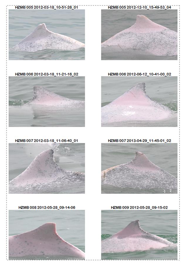
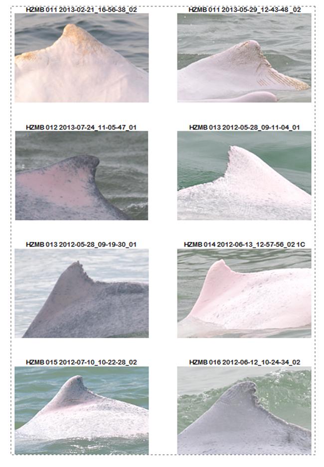
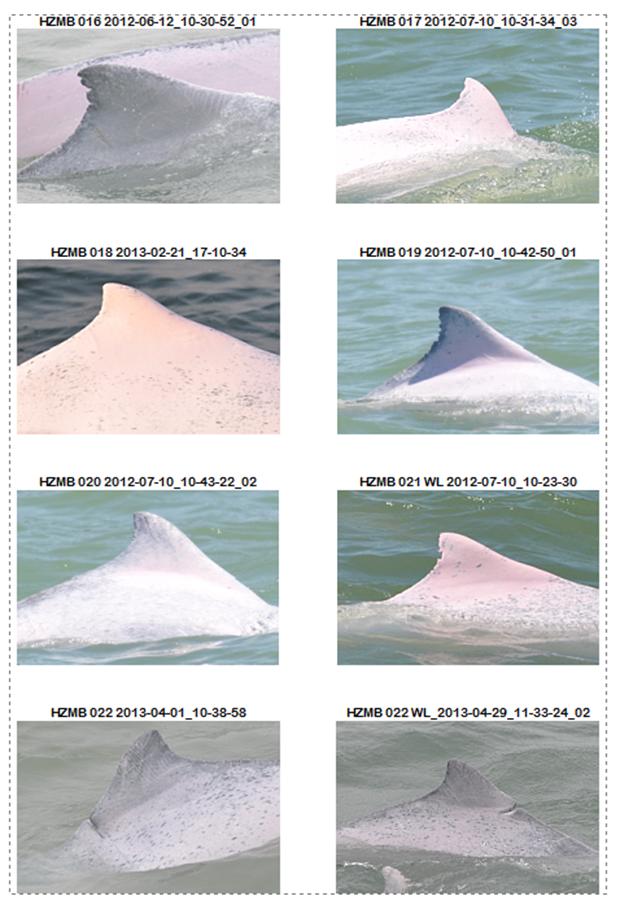


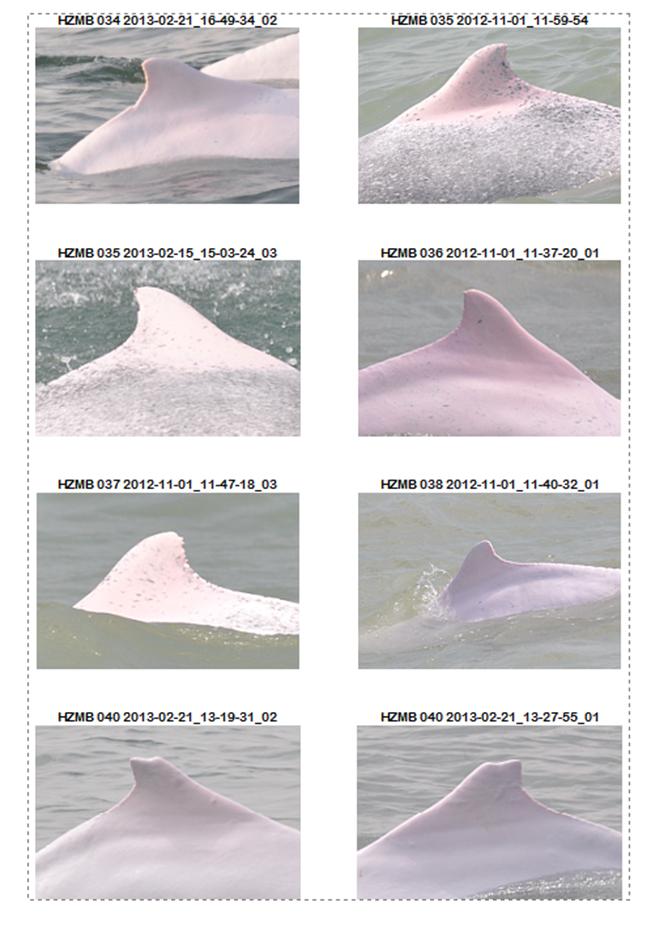
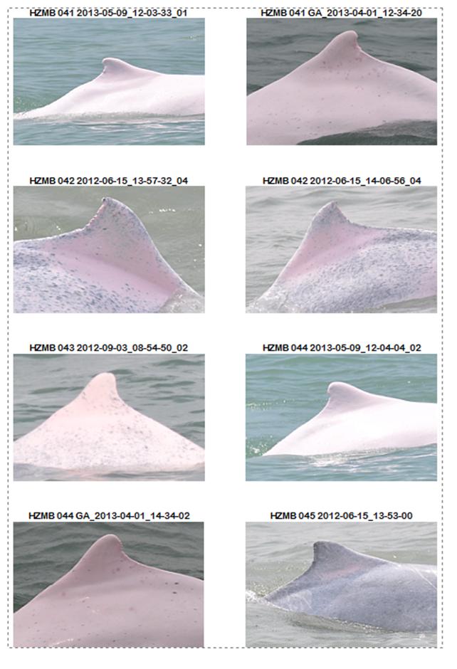
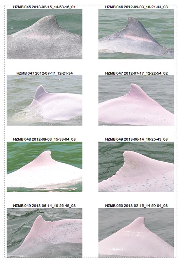

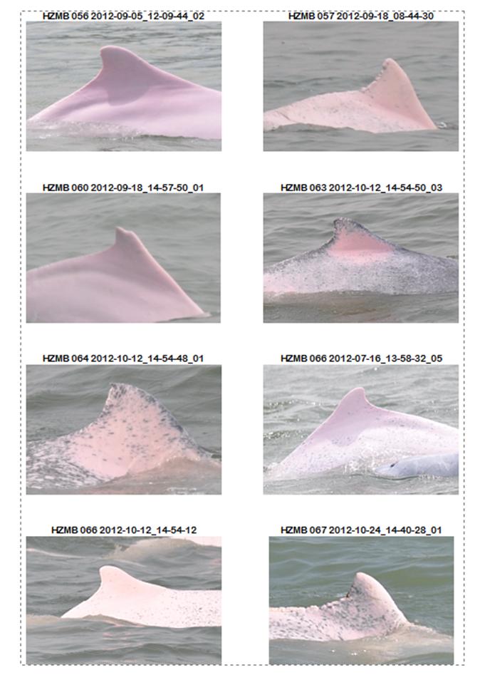
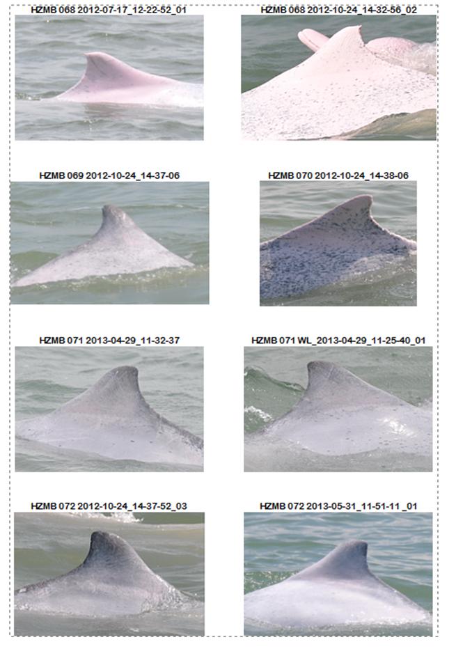
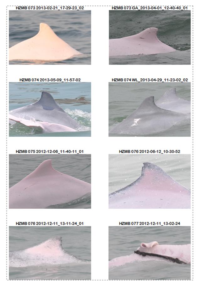
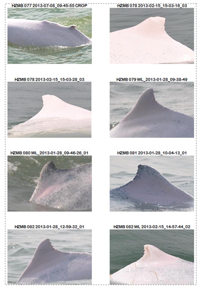
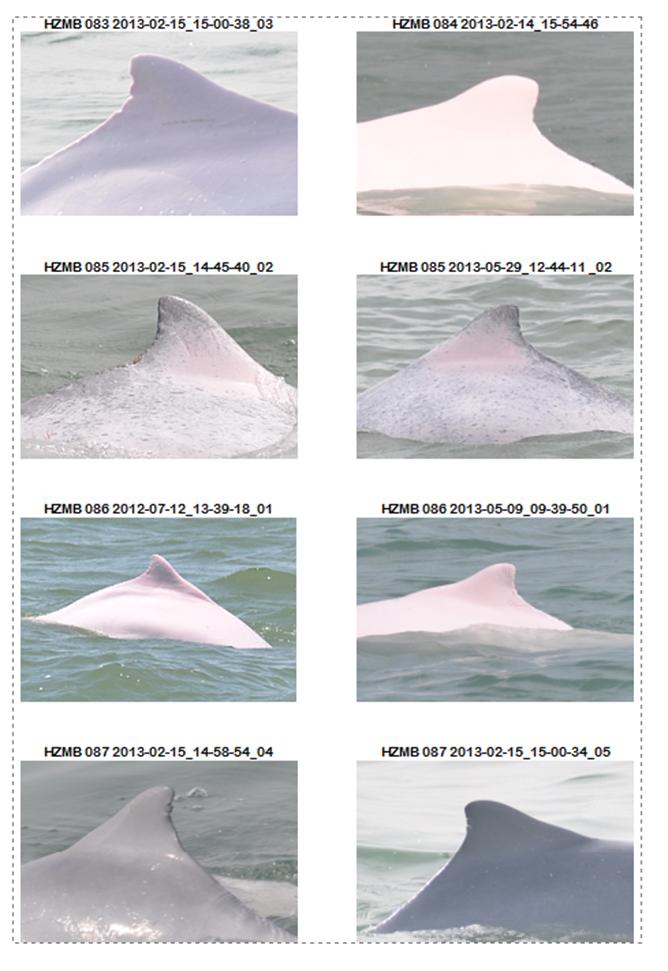
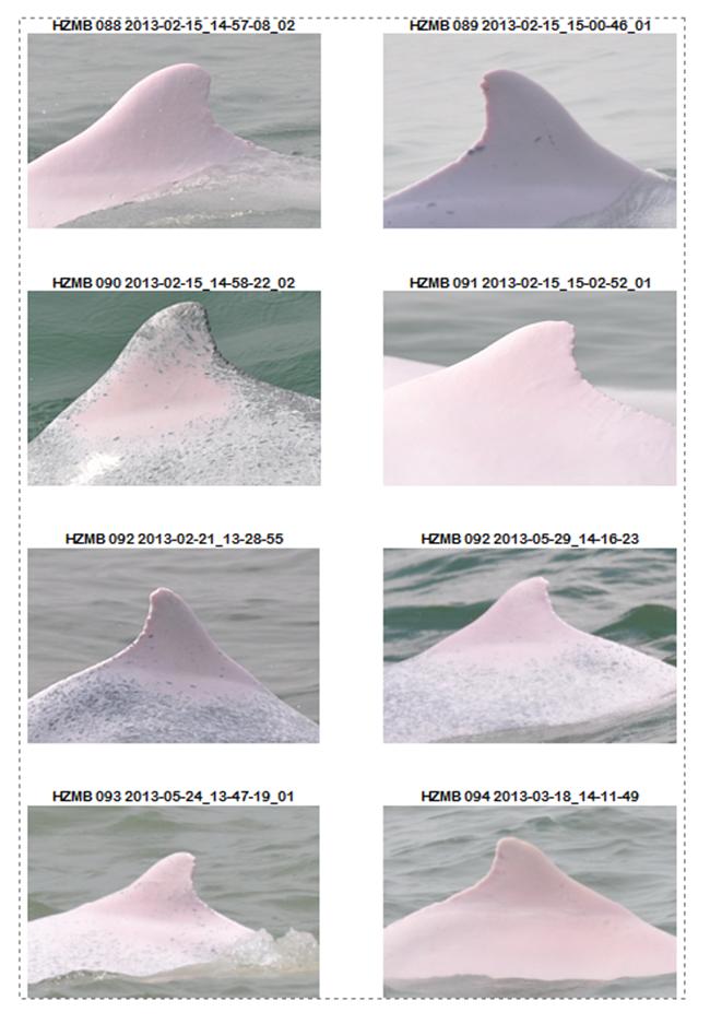
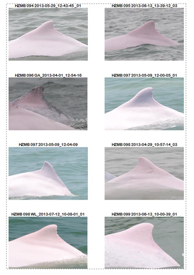
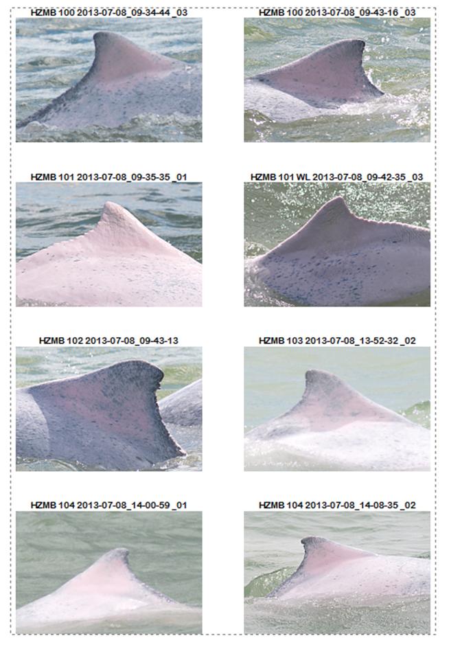
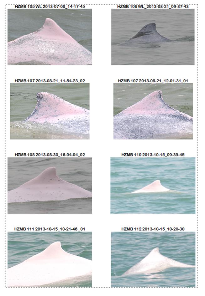
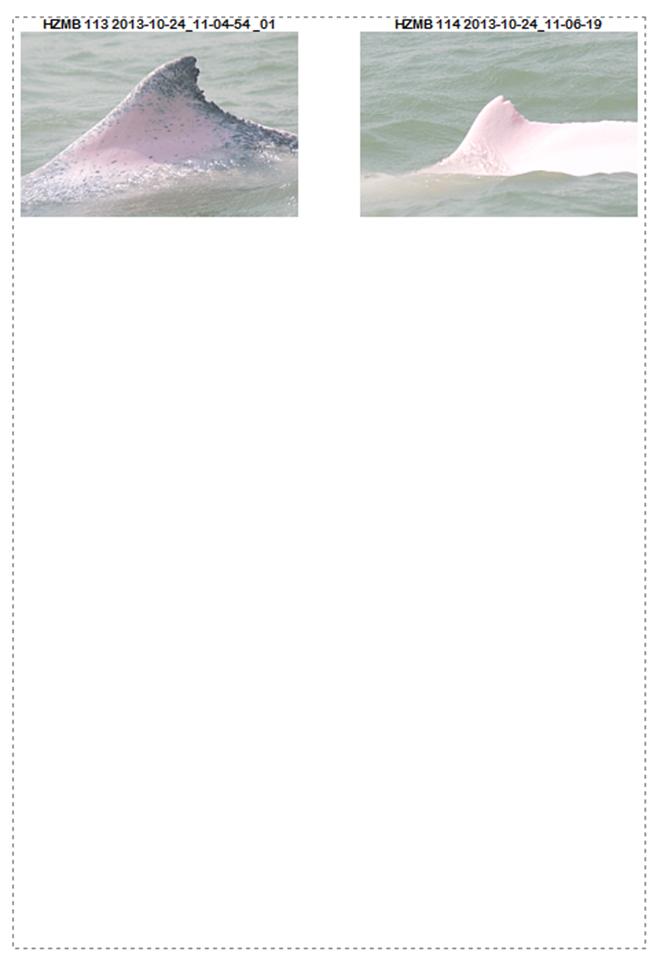
[1]http://www.afcd.gov.hk/english/conservation/con_mar/con_mar_chi/con_mar_chi_chi/con_mar_chi_chi.html
[2] Logger is purpose built software which automatically collects and stores GPS data and contains a user configurable interface for the manual entry of the data required for line transect and other cetacean research studies (Gillespie et al 2010).
[3] Group size is defined as an aggregation of dolphins within 100m of each other involved in similar behaviour (Connor et al 1998).
[4] During sightings a minimum, maximum and best estimate of group size is noted; the range stated represents the minimum and maximum numbers estimated)
[5] Updated data set provided April 2013
[6] The provision of data from multiple government agencies and the private
sector is acknowledged
[7]
Please note: the monthly report for October 2013
erroneously reported no calves were seen during this month. There were four
sightings of calves during this month.
[8] Scott Hayward, L. A. S. , Mackenzie ,M. L. , Donovan, C R , Walker, C. & Ashe, E. (2013), Complex Region Spatial Smoother (Cress). Journal of Computational and Graphical Statistics. In press
[9] http://www.snh.gov.uk/docs/a609642.pdf
[10] Paxton, C., Mackenzie, M. L., Burt, L., Rexstad, E. & Thomas, L. (2011) Phase II Data Analysis Of Joint Cetacean Protocol Data Resource, Http://Jncc.Defra.Gov.Uk/Pdf/Jcp_Phase_II_Report.Pdf
[11] Comparing Pre- and Post-Construction Distributions of Long-Tailed Ducks Clangula Hyemalis in and Around the Nysted Offshore Wind Farm, Denmark : A Quasi-Designed Experiment Accounting for Imperfect Detection, Local Surface Features and Autocorrelation. Http://Hdl.Handle.Net/10023/2008
[12] Hardin, J. W. and Hilbe, J., Generalized Estimating Equations. 2003. Chapman & Hall/CRC Press.
